 Basem Rajjoub
3D stress analysis: Mohr's circles — interactive tool and Asymptote script
Contents
Given a full 3D stress tensor, this post provides an interactive browser tool to compute principal stresses and plot the three Mohr’s circles, along with Von Mises and Tresca values. The same computation is also available as an Asymptote script for publication-quality PDF output.
Interactive Tool
Theory
The stress tensor
The state of stress at a point in a 3D body is fully described by the symmetric Cauchy stress tensor $\boldsymbol{\sigma}$:
\[\boldsymbol{\sigma} = \begin{pmatrix} \sigma_{11} & \sigma_{12} & \sigma_{13} \\ \sigma_{12} & \sigma_{22} & \sigma_{23} \\ \sigma_{13} & \sigma_{23} & \sigma_{33} \end{pmatrix} = \begin{pmatrix} \sigma_x & \tau_{xy} & \tau_{xz} \\ \tau_{xy} & \sigma_y & \tau_{yz} \\ \tau_{xz} & \tau_{yz} & \sigma_z \end{pmatrix}\]The diagonal entries are normal stresses; the off-diagonal entries are shear stresses. Symmetry ($\sigma_{ij} = \sigma_{ji}$) follows from moment equilibrium, leaving 6 independent components.
Principal stresses
Principal stresses $\sigma_p$ are the eigenvalues of $\boldsymbol{\sigma}$ — the normal stresses acting on planes where shear stress vanishes. They satisfy the characteristic equation:
\[\det(\boldsymbol{\sigma} - \sigma_p \mathbf{I}) = 0\]Expanding the determinant gives the cubic:
\[\sigma_p^3 - I_1\,\sigma_p^2 + I_2\,\sigma_p - I_3 = 0\]where $I_1$, $I_2$, $I_3$ are the stress invariants — scalar quantities that do not change with coordinate rotation (reference):
\[\begin{aligned} I_{1} &= \sigma_{11}+\sigma_{22}+\sigma_{33} \\ I_{2} &= \sigma_{11}\sigma_{22}+\sigma_{22}\sigma_{33}+\sigma_{33}\sigma_{11}-\sigma_{12}^{2}-\sigma_{23}^{2}-\sigma_{31}^{2} \\ I_{3} &= \det(\boldsymbol{\sigma}) = \sigma_{11}\sigma_{22}\sigma_{33}-\sigma_{11}\sigma_{23}^{2}-\sigma_{22}\sigma_{31}^{2}-\sigma_{33}\sigma_{12}^{2}+2\sigma_{12}\sigma_{23}\sigma_{31} \end{aligned}\]The cubic has three real roots (guaranteed for a symmetric real matrix). Using the trigonometric method, they are found via the auxiliary angle:
\[\phi = \frac{1}{3}\cos^{-1}\!\left(\frac{2I_{1}^{3}-9I_{1}I_{2}+27I_{3}}{2\left(I_{1}^{2}-3I_{2}\right)^{3/2}}\right)\]Principal stresses (ordered $\sigma_1 \geq \sigma_2 \geq \sigma_3$):
\[\begin{aligned} \sigma_{1} &= \frac{I_{1}}{3}+\frac{2}{3}\sqrt{I_{1}^{2}-3I_{2}}\,\cos\phi \\ \sigma_{2} &= \frac{I_{1}}{3}+\frac{2}{3}\sqrt{I_{1}^{2}-3I_{2}}\,\cos\!\left(\phi-\frac{2\pi}{3}\right) \\ \sigma_{3} &= \frac{I_{1}}{3}+\frac{2}{3}\sqrt{I_{1}^{2}-3I_{2}}\,\cos\!\left(\phi-\frac{4\pi}{3}\right) \end{aligned}\]Mohr’s circles
Each pair of principal stresses defines one circle in the $(\sigma, \tau)$ plane. The three circles have centers and radii:
\[C_{ij} = \frac{\sigma_i + \sigma_j}{2}, \qquad R_{ij} = \frac{\sigma_i - \sigma_j}{2}\]The outermost circle (between $\sigma_1$ and $\sigma_3$) gives the maximum shear stress $\tau_{\max} = R_{13}$ (Tresca criterion).
Failure criteria
\[\tau_{\max} = \frac{\sigma_1 - \sigma_3}{2} \qquad \text{(Tresca)}\] \[\sigma_{VM} = \sqrt{\frac{(\sigma_1-\sigma_2)^2+(\sigma_2-\sigma_3)^2+(\sigma_1-\sigma_3)^2}{2}} \qquad \text{(Von Mises)}\]Asymptote Script
For publication-quality PDF output, the same computation is available as an Asymptote script. Source on GitHub: BasemRajjoub/Mohr3D.
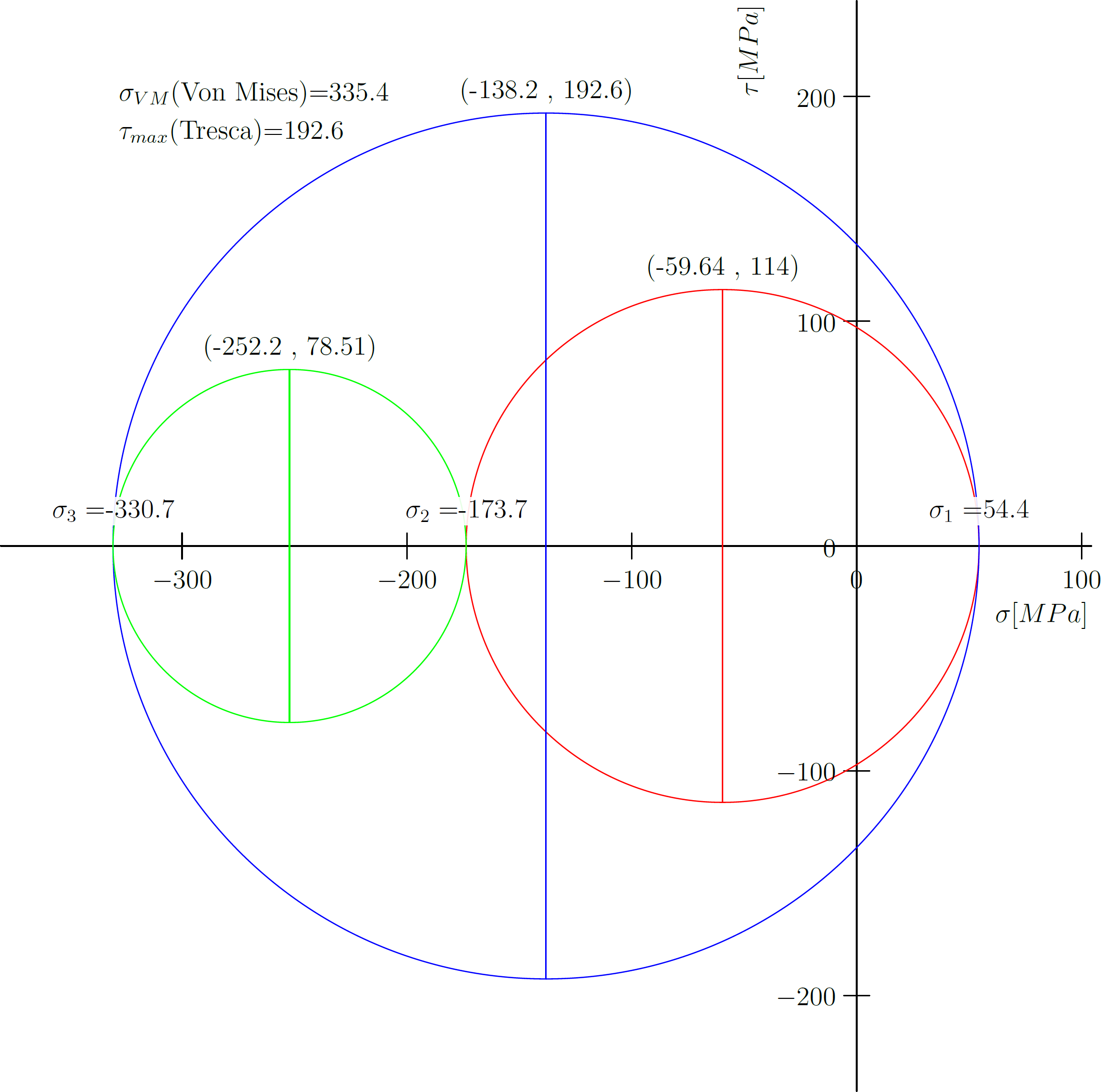 Example output: three Mohr’s circles for a 3D stress state
Set stress tensor components under //Inputs start and run with asy mohr3d.asy — outputs a PDF with the circles, principal stresses, Von Mises, and Tresca values.
| Variable | Description |
|---|---|
s_x, s_y, s_z |
Normal stresses ($\sigma_x$, $\sigma_y$, $\sigma_z$) |
t_xy, t_xz, t_yz |
Shear stresses ($\tau_{xy}$, $\tau_{xz}$, $\tau_{yz}$) |
import graph;
import settings;
settings.outformat = "pdf";

//Inputs start

string m_unit = "MPa";
real unit_step = 100;

real s_x = -100;
real s_y = -200;
real s_z = -150;
real t_xy = 50;
real t_xz = 100;
real t_yz = 150;

//Inputs end

// Stress Invariants
// https://en.wikiversity.org/wiki/Introduction_to_Elasticity/Principal_stresses

real I_1 = s_x+s_y+s_z;
real I_2 = s_x*s_y+s_y*s_z+s_z*s_x-t_xy**2-t_xz**2-t_yz**2;
real I_3 = (s_x*s_y*s_z)-s_x*t_yz**2-s_y*t_xz**2-s_z*t_xy**2+(2*t_xy*t_xz*t_yz);

real phi = (1/3)*acos((2*I_1**3-9*I_1*I_2+27*I_3)/(2*(I_1**2-3*I_2)**(3/2)));

// Principal Stresses

real s_1 = (I_1/3)+(2/3)*sqrt(I_1**2-3*I_2)*cos(phi);
real s_2 = (I_1/3)+(2/3)*sqrt(I_1**2-3*I_2)*cos(phi-2*pi/3);
real s_3 = (I_1/3)+(2/3)*sqrt(I_1**2-3*I_2)*cos(phi-4*pi/3);

// Circles

real C_1 = 0.5*(s_1+s_2);
real C_2 = 0.5*(s_1+s_3);
real C_3 = 0.5*(s_2+s_3);

real R_1 = 0.5*(s_1-s_2);
real R_2 = 0.5*(s_1-s_3);
real R_3 = 0.5*(s_2-s_3);

path c1 = circle((C_1,0),R_1);
path c2 = circle((C_2,0),R_2);
path c3 = circle((C_3,0),R_3);

draw(c1,red);
draw(c2,blue);
draw(c3,green);

draw((C_1,R_1)--(C_1,-R_1),red);
draw((C_2,R_2)--(C_2,-R_2),blue);
draw((C_3,R_3)--(C_3,-R_3),green);

xaxis(L="$\sigma ["+m_unit+"]$", axis=YZero, xmin=s_3-50, xmax=s_1+50, ticks=Ticks(Step=unit_step));
yaxis(L="$\tau ["+m_unit+"]$", axis=XZero, ymin=-R_2-50, ymax=R_2+50, ticks=Ticks(Step=unit_step));

label(L="$\sigma_1="+format(s_1)+"$", position=(s_1,0), N*3, filltype=Fill(white+opacity(0.9)));
label(L="$\sigma_2="+format(s_2)+"$", position=(s_2,0), N*3, filltype=Fill(white+opacity(0.9)));
label(L="$\sigma_3="+format(s_3)+"$", position=(s_3,0), N*3, filltype=Fill(white+opacity(0.9)));

label(L="$("+format(C_1)+"\ ,\ "+format(R_1)+")$", position=(C_1,R_1), N);
label(L="$("+format(C_2)+"\ ,\ "+format(R_2)+")$", position=(C_2,R_2), N);
label(L="$("+format(C_3)+"\ ,\ "+format(R_3)+")$", position=(C_3,R_3), N);

real s_vm = sqrt(0.5*((s_1-s_3)**2+(s_2-s_3)**2+(s_1-s_2)**2));

label(L="$\sigma_{VM}$ (Von Mises)="+format(s_vm), position=(s_3,R_2), NE);
label(L="$\tau_{max}$ (Tresca)="+format(R_2), position=(s_3,R_2), SE);